Reading the wells before they show their hand with machine learning
The outcome we're after.
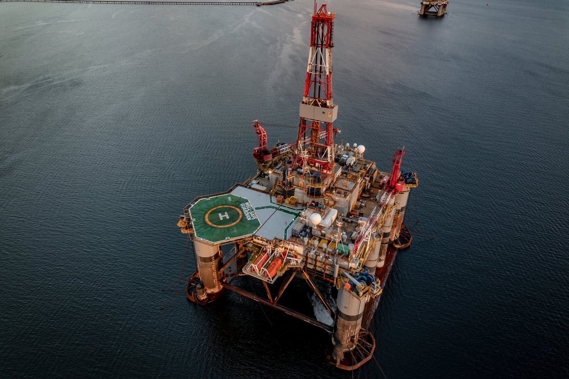
An oilfield services firm lives or dies on when it intervenes. Every well throws off pressure, temperature and flow readings by the second, and somewhere in that stream a well is quietly starting to decline. Caught late, it costs lost production and a scramble. A machine learning model on Databricks reads the high-frequency sensor and production history across the whole field, forecasts what each well should do, and flags the ones drifting off track early enough to plan a response rather than react to one.
Book a discovery call The decline an oilfield services firm spots too late
An oilfield services firm is judged on the wells it keeps producing, and the hardest part is timing. Every well streams pressure, temperature and flow readings by the second, and produced volumes pile up day after day. Somewhere in that flood, a well is starting to decline. The question is whether the firm sees it in time to plan a response or finds out from a month-end report once the production has already been lost.
The usual review cadence works against early detection. Production engineers look at a well’s numbers periodically, often monthly, across a field of hundreds of wells. A slow, gradual decline hides easily inside normal variation when you only glance at it now and then, and by the time it is obvious on a chart, weeks of output are gone. The firm ends up reacting to declines instead of planning ahead of them, sending crews out in a scramble rather than scheduling a job around safety, equipment and the rest of the field.
Spreadsheets and dashboards do not close the gap on their own. The data volume is the first wall. High-frequency readings across a whole field run to billions of rows, far past what a spreadsheet or a single database query handles comfortably. The data is also messy. Sensors drop out and report nonsense, wells are shut in for planned work, and intervals are irregular. A naive view of all this confuses a dead sensor or a planned shut-in with a real production drop, so the firm cannot trust what it is looking at. Reading the field early needs both the scale to process it and the care to handle what the raw numbers do not say. Operations and safety planning depend on getting this right, and well data is handled under the firm’s own confidentiality and operational controls.
Why Databricks for messy well time-series
The aim is one forecast per well, refreshed across the whole field, that engineers can trust enough to plan around. We headline these builds on Databricks because well data is exactly the big, irregular, time-series problem its lakehouse design handles well, and because a forecast nobody can reproduce is a forecast nobody acts on.
Databricks ingests the high-frequency sensor and production streams from every well into one lakehouse, so the raw readings, the cleaned series and the engineered features live in the same governed place rather than scattered across exports. Apache Spark does the heavy lifting underneath, processing billions of rows and engineering features across the full field in parallel instead of well by well, which is what makes a daily refresh across hundreds of wells practical. On top of that, MLflow tracks every model, its features and the data it was trained on, so a forecast can be reproduced and explained later. In a field where a model is telling an engineer to send a crew, reproducible and explainable is not a nicety.
We engineer features that describe each well’s behaviour, such as recent decline rate, pressure and flow trends and time since the last intervention, then train models that forecast expected production and surface the wells running below it. Each well is baselined against its own normal, so a naturally modest producer is judged on its own terms rather than against the strongest well in the field. The whole platform runs on Microsoft Azure in an Australian region, so the firm’s operational data stays in a controlled environment under its own access rules.
We kept the data layer and the modelling deliberately separate. Well data at this scale punishes shortcuts, and a clean lakehouse feeds reservoir and equipment-health work later, not just today’s production forecast.

Building it, and where it got hard
The model was rarely the hard part. The friction lived in the data, and one problem is almost guaranteed to bite. The field is full of things that look like decline but are not.
Early in the build the model flagged a cluster of wells as declining sharply. They were not. Some had been shut in for planned maintenance, so production dropped to zero by design, and the model read a deliberate stop as a collapse. Others had a faulty sensor reporting drifting or dead values, which the model took at face value. False alarms like these are worse than no alarm. Send a crew to a healthy well a few times and the engineers stop trusting the system, which is the fastest way to kill a forecasting tool.
The fix was less about a cleverer model and more about teaching it the difference between a real decline and an artefact. We used Databricks and Spark to process the full volume and to detect and mask sensor faults, so dead or drifting readings were not fed in as genuine production. Shut-in periods were identified and handled explicitly, so a planned stop was treated as a stop rather than as decline. Each well was baselined against its own history so its normal variation was understood before any drift was called. Then we validated every model on held-out time periods rather than scoring it on the data it had seen, with MLflow tracking each run so a forecast could be reproduced and defended. A model that only looks accurate on its training window is the easiest trap in time-series work, and held-out validation is how you avoid shipping it.
One more constraint shaped the build. Refresh windows were sized so the daily run across the whole field finished well before the engineers logged on, because a forecast that lands after the morning planning meeting helps nobody.
What changed
In a representative build the forecasts tracked actual production closely enough across the validation window that engineers used them to plan rather than treating them as a rough guess. Genuine decline was flagged weeks earlier than the previous monthly review had caught it, which turned a reactive scramble into a job the firm could schedule around crews, safety and the rest of the field. Just as important, shut-ins and sensor faults stopped triggering false alarms, so the team spent its time on wells that were actually drifting instead of chasing dropouts in the data.
These figures are illustrative. They describe the pattern we see rather than a published result for a named firm. The shape is the point. The signal that was always buried in the sensor stream reaches the engineers while there is still time to act, the field is watched continuously instead of glanced at monthly, and an intervention becomes a planned decision rather than a response to lost production.
Where this fits
Production forecasting is one application of our Artificial Intelligence service, built on Databricks, for the mining, oil and gas sector. It is a contained, high-return starting point, because the sensor and production data already exists and the value comes from processing it at scale and modelling it carefully enough to trust. If you are finding out about declining wells from a monthly report, the place to start is to map your sensor and production data and decide where an early flag would change what your engineers do next.
Representative outcomes
Forecast accuracy
In a representative build, per-well production forecasts tracked actuals closely enough over the validation window to be trusted for planning rather than treated as a rough guide.
Earlier decline detection
Genuine decline was flagged weeks earlier than the engineers' previous monthly review caught it, giving real time to plan an intervention.
Fewer false alarms
Shut-ins and sensor faults were no longer read as decline, so the team chased real problems instead of dropouts in the data.
This solution applies our Artificial Intelligence service, built primarily on Databricks , for the Mining, Oil & Gas sector.
Supporting stack: Apache Spark, Microsoft Azure.
Related solutions.
Representative Solution. An illustrative scenario based on how we deliver, not a named client engagement. Outcome figures are representative, not published results.
Frequently asked.
How is machine learning used in oil and gas and mining?
What is predictive analytics in oil and gas?
What data does a well production forecast actually need?
How does one model handle many wells that behave differently?
How does the firm act on a forecast once a decline is flagged?
See your wells decline before they cost you
We will map your sensor and production data and show you how a forecasting model would flag a declining well early enough to plan the intervention.
Book a discovery call